


Calculating RPM Parameters from Load Forecast Model Output
This section contains descriptions of the R-scripts that calculate statistical parameters from outputs of the Council’s load forecast model to become input into the Council’s Regional Portfolio Model (RPM).
More specifically, the load forecast model produces hourly weather-normalized load forecasts for three levels: high, medium, and low (Method to Forecast Climate Change Loads for more details). The three levels of load are forecasted for future years of interests, for example, the 30 years from 2020 to 2049. Since the RPM uses four quarterly time-steps in a year, then one of the R-scripts first calculates quarterly averages for the 3 levels of hourly loads. Then it performs a linear model regression fit between the yearly index and the log of the ratio of the quarterly averaged high loads to the quarterly averaged medium loads. The R-script also develops a linear regression model for the log of the ratio of the quarterly averaged medium loads to the quarterly averaged low loads. The linear regression coefficients are inputs into the RPM.
The load forecast model also produces hourly temperature-sensitive multipliers (Method to Forecast Climate Change Loads for more details). The other R-script then calculates hourly temperature-sensitive loads from the medium weather-normalized load forecast and the temperatures-sensitive multipliers. From the hourly temperature-sensitive loads, the R-script then calculates a yearly average for each of the 30 years. Then for each of the 120 quarters, the script resamples (with replacement) the hourly temperature-sensitive loads within that quarter and calculates a quarterly averaged load. For each quarter, the resampling and calculation of the quarterly averaged load are done multiple times. Finally, for each quarter, from the distribution of quarterly averaged loads resulting from the multiple resamplings, the standard deviation of the log of the ratio of quarterly averaged load to yearly averaged load is calculated. The standard deviations for all 120 quarters become inputs into the RPM.
The Linear Regression Coefficients
The load model has as inputs the forecasted regional temperatures from three selected RMJOC climate scenarios, A, C and G, for the 30 years from 2020 to 2049 (see climate change scenarios selection write-up for more details). Then from the forecasted temperatures for a climate scenario, monthly cooling-degree-days (CDDs) and heating-degree days (HDDs) are calculated and used to derive the monthly weather-normalized Northwest regional loads for a selected year (e.g., 2025, 2031). The average of the 30 years of forecasted temperatures (as determined within the load model) is then used to transform the monthly weather-normalized loads into the hourly weather-normalized loads for the selected year.
To simulate operations of the Northwest power system for an operating year, three levels of hourly weather-normalized loads are calculated: the high, medium, and low load forecasts. For convenience for the Power Plan, the weather-normalized loads were calculated for all 30 years, from 2020 to 2049. An example portion of the weather-normalized loads for climate scenario A (see summary of climate change scenario write-up) for pathways to decarbonization studies is presented in Figure 1.
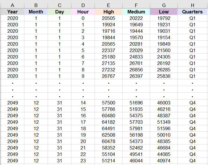
Figure 1: An example weather-normalized loads with high, medium, and low forecasts for 2020 to 2049 for pathways to decarbonization studies. The four quarters for each year are listed in column H.
In Figure 1, columns A to D list the years, months, days, and hours for the high, medium, and low forecasts of the weather-normalized loads, in units of MW, in columns E to G, respectively. For convenience, leap days are not included in columns A to D. Thus, there are 262,800 rows of data for the 30 years of hourly loads. In addition, the four quarters for each year, Q1, Q2, Q3, and Q4 are listed in column H.
The R-script then calculates quarterly averages for each of the high, medium, and low forecasts of hourly loads in columns E to G respectively in Figure 1. Specifically, for each of the 120 quarters in column H, the averages of the hourly loads in columns from E to G are calculated. The results are presented in Figure 2.
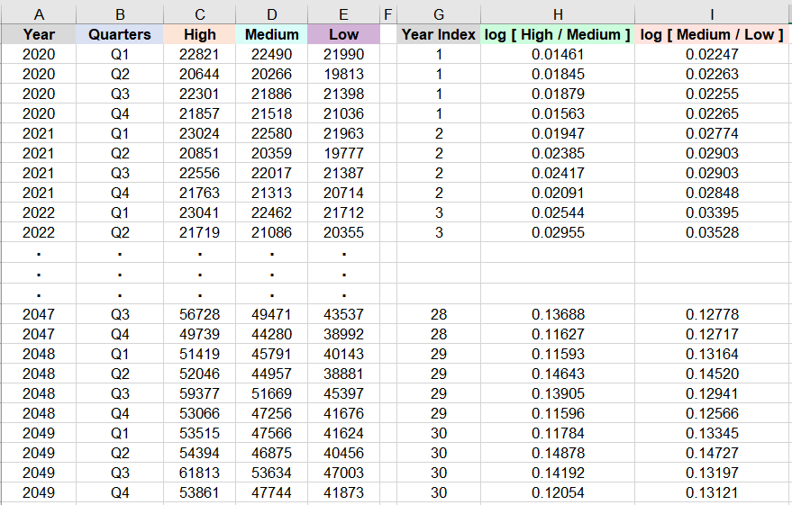
Figure 2: Quarterly averaged weather-normalized loads from Figure 1. In addition, the year index is along column G. Furthermore, the natural log of the ratio of the values in column C to those in column D are calculated in column H, and the natural log of the ratio of the values in column D to those in column E are calculated in column I.
In Figure 2, columns A to B list the years and quarters for the quarterly averaged high, medium, and low forecasts of the weather-normalized loads in columns C to E, respectively. There are 120 rows of data for the 30 years of quarterly averaged loads.
In addition, a year index is added along column G, where for example, the first year, 2020, has index 1 and the thirtieth year, 2049, has index 30. Furthermore, the natural log of the ratio of the quarterly averaged high load forecast (in column C) to the quarterly averaged medium load forecast (in column D) is calculated in column H. Similarly, the natural log of the ratio of the quarterly averaged medium load forecast (in column D) to the quarterly averaged low load forecast (in column E) is calculated in column I.
For simplicity in describing the linear regression model, let the year index in column G be x and the logs of the ratios in columns H and I be yH/M and yM/L respectively. Then the R-script calculates coefficients aH/M, bH/M, cH/M and aM/L, bM/L, cM/L for the corresponding linear regression models:
All the coefficients are then divided by qnorm(0.85) and become inputs into the RPM. While both sets of coefficients are calculated, only one set is used in RPM. In this case we use the ratio between the high and medium load forecast because the distribution of loads above the median load is more pertinent to the questions raised in the RPM. For the example data presented, the coefficients are, aH/M=-5.021×10-5 , bH/M=5.292×10-3 , and cH/M=1.301×10-2 .
For simulating a range of loads RPM generally needs two pieces of information. The loads are assumed to follow a lognormal distribution in each quarter. The medium load forecast sets the center of the distribution which changes from one quarter to the next. This derivation is used to set the range of each of the distributions which can change through time based on the quadratic relationship established by these parameters.
The Standard Deviations
In contrast to the weather-normalized loads used in calculating the regression coefficients in the previous section, the standard deviations are calculated using temperature-sensitive loads. For the RPM, the temperature-sensitive loads are calculated by multiplying the hourly weather-normalized loads in Figure 1 by the corresponding hourly temperature-sensitive multipliers (TSMs). A portion of the hourly TSMs for 2020 to 2049 for climate scenario A is presented in Figure 3.
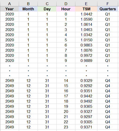
Figure 3: An example TSMs for 2020 to 2049 for pathways to decarbonization studies. The four quarters for each year are listed in column F.
In Figure 3, columns A to D list the years, months, days, and hours for the TSMs in column E. There are 262,800 rows of data for the 30 years of hourly TSMs. In addition, the four quarters for each year, Q1, Q2, Q3, and Q4 are listed in column F.
To calculate temperature-sensitive loads, the other R-script merges the weather-normalized load data in Figure 1 with the TSM data in Figure 3 resulting in Figure 4. For the RPM, only the medium forecast of the weather-normalized loads is used.
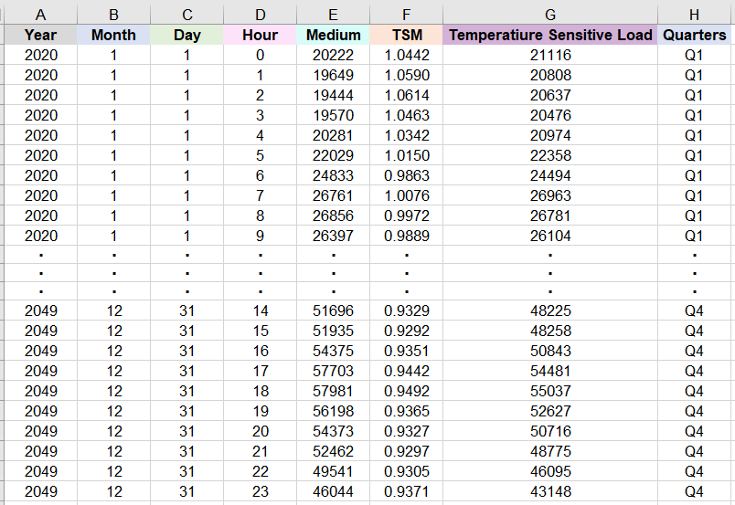
Figure 4: Data set from merging the weather-normalized loads in Figure 1 and the TSMs in Figure 3. The temperature-sensitive loads are calculated in column G.
In Figure 4, columns A to D and H list the years, months, days, hours, and quarters for the medium forecast of the weather-normalized loads in column E and the TSMs in column F. The R-script then calculates the temperature-sensitive loads in column G by multiplying the medium forecast of the weather-normalized loads in column E by the TSMs in column F.
Next, the R-script calculates the yearly averaged temperature-sensitive loads (from column G) for each of the 30 years from 2020 to 2049. The result is presented in Figure 5.
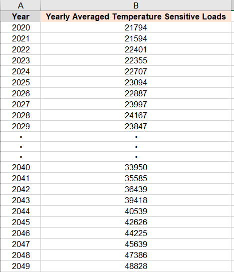
Figure 5: Yearly averaged temperature-sensitive loads for 2020 to 2049 calculated from column G in Figure 4.
Then the R-script merges the yearly averaged temperature-sensitive loads in Figure 5, in units of aMW and denoted by LY , with the hourly temperature-sensitive loads in Figure 4. However, the next set of calculations in the R-script are more easily demonstrated by focusing on data for just 1 of the 120 quarters of the merged data set. For this example calculation, the relevant merged data for quarter Q1 and year 2025 are presented in Figure 6.
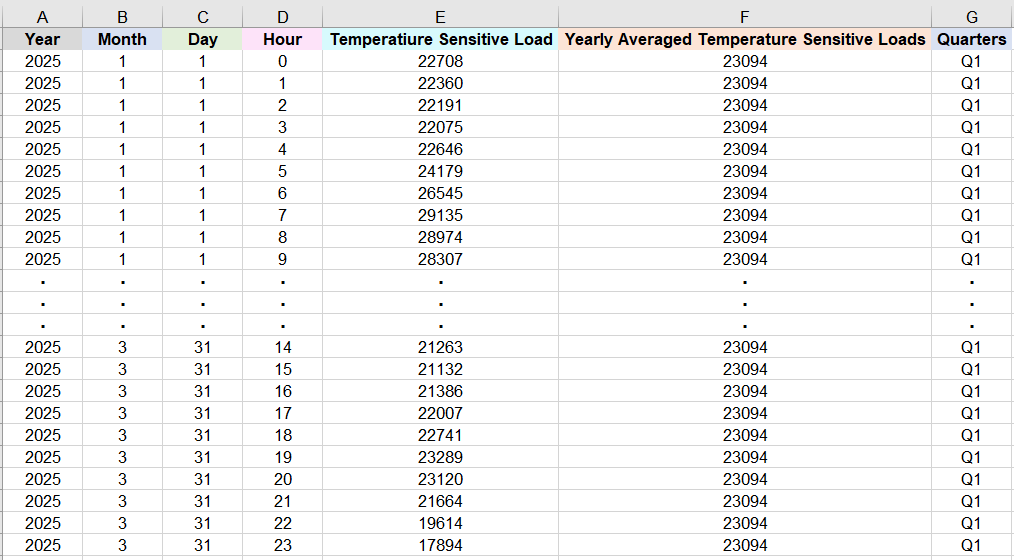
Figure 6: The quarter Q1 and year 2025 portion of the data set from merging the hourly temperature-sensitive loads in column G in Figure 4 and the yearly averaged temperature-sensitive loads in Figure 5.
In Figure 6, for quarter Q1 and year 2025, the columns A to D and G list the year, months, days, hours, and quarter for the medium forecast temperature-sensitive loads in column E. For quarter Q1, there are 2,160 rows of hourly data. In addition, from Figure 5, the yearly averaged load for 2025 is 23,094 aMW and listed along column F in Figure 6.
Then the 2,160 rows of hourly data for quarter Q1 and year 2025 in Figure 6 are resampled with replacement. After the resample, , the (quarterly) average of the 2,160 hourly medium forecast temperature-sensitive loads in column E, is calculated. Also calculated is
, representing the natural log of the ratio of the quarterly averaged load to the yearly averaged load.
For inputs into the RPM, there are 10,000 resamplings. Therefore, there are 10,000 values of the natural logs of the ratios which are represented by the set where index i represents the i -th resample. Then the standard deviation is calculated for this set, which also represents the standard deviation for quarter Q1 of year 2025.
The same processes of 10,000 resamplings followed by calculation of the standard deviations for are performed for the remaining 119 quarters. The R-script implements the various calculational steps for the standard deviations as described. For the example data, the result is presented in Figure 7.
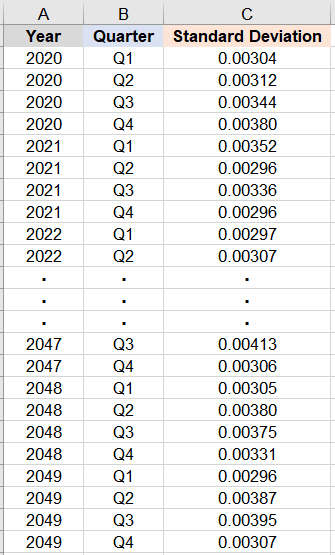
Figure 7: Standard deviations for the 10,000 resamplings for each quarter and each year from 2020 to 2049.
In Figure 7, columns A to B list the years and quarters for the standard deviations in column C. For the example data presented, the 120 rows of quarterly standard deviations become inputs into the RPM.
In RPM the annual weather-normalized loads simulated are translated into quarterly temperature-driven shapes using the ratio of the quarterly average temperature-based load to the annual weather-normalized load. The standard deviations derived from this method are used to add variation to these quarterly ratios allow for RPM to have a range of potential quarterly loads and as a consequence a range of potential annual average loads for a given weather-normalized annual average load.