


Market Supply
The regional power supply has access to two separate market supplies for energy. The first source is from neighboring regions who often have excess generating capacity during their non-peak seasons. For example, because California’s peak demands occur in summer, it should have surplus generating capability during winter, when the Northwest generally has its highest peak demands. Historically, the California market supply has been relatively expensive because marginal resources (next cheapest resources to operate) have typically been coal or gas-fired generators. Thus, most often the California market was used for adequacy needs in the Northwest.
However, enactment of West-wide clean air laws and policies, are leading to a very large buildout of renewable resources, in particular solar generation. Because of the anticipated high amount of new solar generating capability, the magnitude and price of the Southwest market is expected to change. Electricity pricing models show greater amounts of Southwest market supply, with mid-day prices dropping to very low or negative values. This expected change in the out-of-region market means that it will be accessed not only for Northwest adequacy needs but also for economic opportunities when market prices are below regional resource operating costs (including hydro). Market prices are expected to be lowest during the hours after the California morning demand ramp and before its evening ramp (as solar generation diminishes). Highest market prices are expected during a 2-hour morning period and during a 6-hour evening ramp period (see figure below).
Illustration of California Market Prices in Summer

The figures below show redeveloped GENESYS results for average energy imported over each hour of the day and maximum energy imported over each hour of the day in December and August. Please note that the scales in the charts below are different. Imports in December are limited to a maximum of 2,500 megawatts per hour and in August to a maximum of 1,250 megawatts per hour. These limitations are recommended by the Resource Adequacy Advisory Committee.
Average and Maximum Hourly Imported Energy

|

|
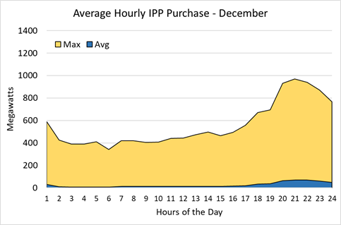
The second source of market supply is from regional independent power producers (IPP). The in-region market is mostly comprised of gas-fired generators with an aggregate nameplate capacity of about 2,400 megawatts. Even though these resources are physically located within the Pacific Northwest region, their generation is available to anyone. Figures below show the redeveloped GENESYS results for average and maximum hourly energy purchased from IPP resources in December and in August. On average (blue area), very little IPP energy is purchased, however, in the highest hour (out of 180 simulations) IPP generation was about 1,000 megawatts in December and about 1,200 megawatts in August.
Average and Maximum Hourly IPP Energy Purchases
|

|
Hydroelectric System Generation
Aggregate Hydro Generation
Comparing aggregate hydroelectric system generation from the redeveloped GENESYS to results from the classic model and to historic (observed) generation is difficult for many reasons. First, operating constraints do not stay constant over time. For example, operations to improve fish survival have changed significantly over the past decade. Second, historically observed natural river flows are different from climate change projected flows used in the models, both in terms of total volume and seasonal shape. Third, the redeveloped GENESYS treats more hydroelectric projects as reservoirs than do HYDSIM and the classic GENESYS models and, therefore has more useable storage (see section on operating constraints for more detail). Fourth, the new model simulates hydro plant operations hourly, whereas both the classic GENESYS and HYDSIM simulate plant-specific operations monthly. Fifth, the redeveloped GENESYS simulates WECC-wide market transactions, including both imports and exports. The HYDSIM model includes a fixed amount of market sales, and the classic GENESYS does not model out-of-region sales. In addition, there may be other valid reasons why the redeveloped GENESYS aggregate annual and monthly hydro generation should differ from historical data and from the classic model results.
Nonetheless, aggregate hydro generation comparisons have proven to be useful in terms of gauging whether the range in annual and monthly generation from the new model seems reasonable. These comparisons have been presented to both the Resource Adequacy and System Analysis advisory committees and are available here.
Plant Specific Generation
Comparing plant-specific generation from the redeveloped GENESYS to results from the classic model and to historic (observed) generation has the same difficulties as were discussed above. Nonetheless, these comparisons have also proven to be valuable and were presented at the System Analysis Advisory Committee workshop held from August 4th through the 6th. Plant-specific monthly average generation, average spill, average outflow and end-of-month elevation from the redeveloped GENESYS are compared to results from the classic model and to historical data (whenever available). These comparisons are illustrated in three separate interactive spreadsheets [1] [2] [3] that allow the user to select hydro plant and the climate change scenario for comparison.
As discussed in the operating constraints section, resulting end-of-month reservoir contents from the classic GENESYS model were interpolated into end-of-week target contents for the redeveloped GENESYS. This was done in lieu of having to process thousands of monthly hydro operating constraints for the new model. And, with few exceptions, the redeveloped model operates all reservoirs to their target contents within a specified tolerance to ensure that all monthly hydro operating constraints are met in the same order of priority as in the classic model. Occasionally, when comparing end-of-period elevations between the new and classic models (in the spreadsheets identified above), it may appear that target elevations are not met. However, this observation is simply an artifact of the interpolation from end-of-month to end-of-week targets. In most cases, the end-of-month day does not coincide with the end-of-week day.
Plant-specific hourly operations from the redeveloped model are compared to historical data, whenever data was available. Comparisons of the range of operation (generation, outflow, spilled flow, and elevation) are illustrated in the form of envelope graphs that are included in the August 4th workshop. A direct comparison of hourly plant operations for specific time periods can be made by extracting hourly results from the redeveloped GENESYS and obtaining historical operations from this Corps of Engineers site.
Overall, participants at the August 4th workshop appreciated the greater level of detail in the redeveloped GENESYS model’s hydro simulation but generally agreed that it requires more fine tuning. One concern is that the new model seems to have a greater amount of hydro flexibility, that is, a greater within-day range of generation than what has been observed historically. However, it’s possible that a higher range of generation would be expected under anticipated future conditions (climate change flows, shifts in demand and a bigger and less expensive market supply). Nonetheless, all hydro project constraints will be reviewed to ensure that no operations violate prescribed limits. The anticipation is that fine tuning the model will not significantly change the resource adequacy assessment.
Sensitivity Analysis
Early Coal Retirement
A sensitivity study for 2025 with early retirement of Centralia 2, Jim Bridger 2 and North Valmy 2 coal plants (1,331 megawatts) results in less than a one percent increase in LOLP relative to the reference case. This result may seem surprising at first but not when considering the amount of unutilized thermal capacity in the 2025 reference case. It should be noted that the effect of resource retirements on the LOLP can vary significantly in later years due to load growth, changes in market availability and price, continuing climate change trends and other factors.
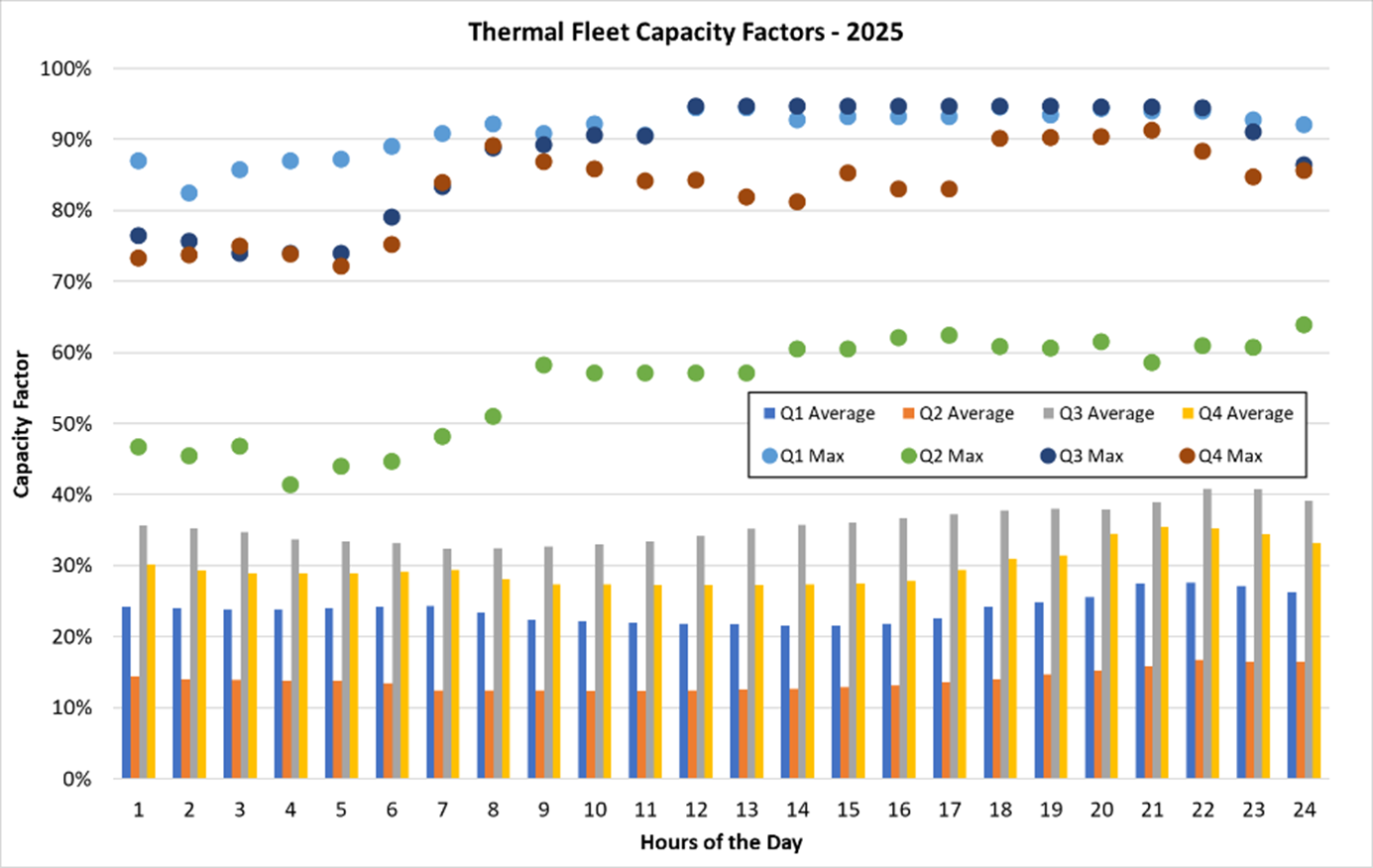
The figures below show thermal fleet average and maximum hourly capacity factors by quarter for both the 2025 reference and early retirement cases. Average hourly capacity factors range from 12 to 50 percent, which translates into a range of 5,400 to 9,500 megawatts of unutilized capacity for the non-retired thermal plants – much more than is needed to offset retired coal plant capacity. However, comparing expected availability of unused thermal capacity to the fixed amount of retired capacity does not provide a good indication of how resource adequacy is affected.
A better gauge of the coal retirement’s effect on adequacy is to examine the availability of unused thermal capacity during hours with the highest capacity factors. Maximum hourly capacity factors can be used to assess the minimum amount of unutilized hourly thermal capacity. For the reference case, the maximum hourly capacity factors are 93, 82, 92 and 93 percent for quarters 1 through 4, respectively. That translates into about 900 megawatts of unutilized thermal capacity in quarters 1, 3 and 4 and into about 2,300 megawatts in quarter 2. The 900 megawatts of unutilized thermal capacity in quarters 1, 3 and 4 are not quite enough to cover the 1,331-megawatt capacity loss from retirement – but the gap (of about 400 megawatts) is only for one hour out of approximately 400,000 simulated hours per quarter (180 simulations). Based on these data, one might qualitatively conclude that the effect of coal retirement on the LOLP may not be as severe as first thought due to the high availability of unutilized thermal capacity. Of course, the most accurate assessment of the impact to resource adequacy is to run the 2025 case with the three named coal plants removed, which results in an LOLP of 0.6 percent, as noted above.
Thermal Fleet Hourly Capacity Factors by Quarter

Non-stochastic Forced Outage Rates
Another concern, raised by members of the Council’s advisory committee, is that the redeveloped GENESYS does not model generator forced outages stochastically and, therefore, is overestimating adequacy (i.e., underestimating LOLP). Currently, the model simply derates generating resource capacity by an average forced outage rate of 5.9 percent. This is a valid concern because thermal system forced outage rates will often exceed 5.9 percent, which could lead to shortfall events. The probability density function for aggregate system forced outage rates generally follows a Weibull distribution. A Weibull distribution is like a normal distribution but has a shorter and steeper curve from zero to the mean value, followed by a flatter and longer tail-end distribution. From past studies using the classic GENESYS (which models forced outages stochastically), aggregate system forced outage rates for the regional thermal fleet range from zero (unlikely), to an average of about 6 percent, to a high of 25 percent or greater (very unlikely). The regional thermal fleet has about 150 plants, so an aggregate forced outage rate of 25 percent means that one quarter of the fleet or about 37 plants would be out of service during a particular hour. We have observed aggregate forced outage rates that high in classic GENESYS simulations, but they occur infrequently relative to the number of simulated hours.
The redeveloped GENESYS has the infrastructure to model forced outage rates stochastically, but due to run-time constraints (i.e., to allow studies to complete overnight), a decision was made to use a flat outage rate for these studies. It is difficult to guess how the LOLP might change if forced outages are modeled stochastically. However, results from the early coal retirement study described above can provide some perspective. Removing 1,331 megawatts of thermal capacity is equivalent to increasing the flat forced outage rate from 5.9 to 16.9 percent. That means that a flat 16.9 percent forced outage rate would theoretically increase the LOLP by less than one percent in 2025. This may also seem surprising at first but, as with the early coal retirement case above, there appears to be sufficient unutilized thermal fleet capacity in 2025 to offset the lost capacity. Unfortunately, this does not explicitly answer the question. Given that the aggregate forced outage rate could be higher than 16.9 percent, it is possible that modeling outages stochastically would result in a higher LOLP. The Council will continue to investigate this.
Effects of High Load Growth
The Council’s capital expansion model examines a 20-year study horizon with a very wide range of load variation. However, to capture the effects of an accelerated load growth, the Council analyzed a future scenario with much higher loads tied to actions aimed at reaching a high level of decarbonization. As anticipated, resource needs for the decarbonization scenario were greater. The Council used these results along with results from all other scenarios to develop its resource development plan.
However, it is often important to understand how a specific parameter can affect adequacy in isolation. Toward that end, we can again refer to the 2025 early coal retirement study to get a sense of how a higher level of demand can affect adequacy. In that sensitivity study, the removal of 1,331 megawatts of thermal capacity can be interpreted as being equivalent to raising demand in every hour by 1,331 megawatts – at least it is a fair approximation. Increasing the expected winter peak load of 32,600 megawatts by 1,331 megawatts represents about a 4 percent increase in peak load. This means that a 4 percent increase in peak load (in 2025) is estimated to increase the LOLP by less than one percent. It should be noted that the effect of higher loads on adequacy can vary significantly in later years due to overall load growth, changes in market availability and price, continuing climate change trends and other factors.